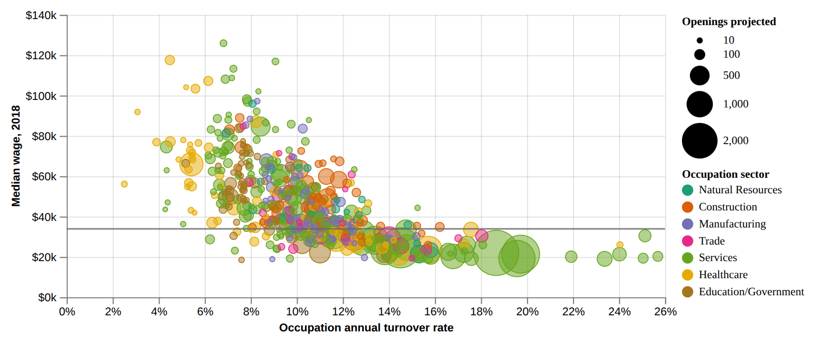
Job Projections
Load and prepare data
# Source : https://observablehq.com/@eidietrich/mt-dept-labor-industry-job-growth-projections-2018-2028?collection=@observablehq/finance-and-strategy
import json
from collections import namedtuple
from pathlib import Path

import detroit_live as d3
import polars as pl
import requests

URL = "https://gist.githubusercontent.com/eidietrich/0047db2bfcfae1543ff37c70474587d3/raw/51bcb25225d5517c40fc8328645973183ed140e6/trimmed-for-vis.json"
Margin = namedtuple("Margin", ("top", "right", "bottom", "left"))

PWD = Path(__file__).resolve().parent
STYLE_PATH = PWD / "styles" / "job_projections.css"

# Download data if not found else load data from `examples/data` folder
def load_data() -> pl.DataFrame:
    data_path = PWD / "data"
    if data_path.exists():
        path = data_path / "trimmed-for-vis.csv"
        if path.exists():
            return pl.read_csv(path)
    data_path.mkdir(exist_ok=True)
    df = pl.from_dicts(json.loads(requests.get(URL).content))
    df.write_csv(data_path / "trimmed-for-vis.csv")
    return df


# Prepare data processing
color_domain = [
    "Natural Resources",
    "Construction",
    "Manufacturing",
    "Trade",
    "Services",
    "Healthcare",
    "Education/Government",
]
color_range = [
    "#1b9e77",
    "#d95f02",
    "#7570b3",
    "#e7298a",
    "#66a61e",
    "#e6ab02",
    "#a6761d",
]

sector_cats = {
    "Marketing": "Services",
    "Business Management & Administration": "Services",
    "Health Science": "Healthcare",
    "Hospitality & Tourism": "Services",
    "Architecture & Construction": "Construction",
    "Transportation, Distribution & Logistics": "Trade",
    "Human Services": "Healthcare",
    "Education & Training": "Education/Government",
    "Manufacturing": "Manufacturing",
    "Finance": "Services",
    "Agriculture, Food & Natural Resources": "Natural Resources",
    "Law, Public Safety, Corrections & Security": "Services",
    "Information Technology": "Services",
    "Arts, Audio/Video Technology & Communications": "Services",
    "Government & Public Adminstration": "Education/Government",
    "Science, Technology, Engineering & Mathematics": "Services",
}

clean_ed_level = {
    "No formal educational credential": "High school diploma or less",
    "High school diploma or equivalent": "High school diploma or less",
    "Some college, post-HS training or Associate's degree": "Some college or two-year degree",
    "Bachelor's degree": "Four-year degree",
    "Master's degree": "Graduate degree",
    "Doctoral or professional degree": "Graduate degree",
}


ed_order = {value: i for i, (key, value) in enumerate(clean_ed_level.items())}
ed_order["High school diploma or less"] = 0

# Data processing
df: pl.DataFrame = (
    load_data()
    .with_columns(
        pl.col("sector").replace_strict(sector_cats).alias("sector_cat"),
        pl.col("ed_level").replace_strict(clean_ed_level).alias("ed_level"),
    )
    .with_columns(
        pl.col("ed_level").replace_strict(ed_order).alias("ed_level_order"),
        pl.col("Annual Openings 2018-2028").round().alias("openings"),
        (
            (pl.col("Annual Exits 2018-2028") + pl.col("Annual Transfers 2018-2028"))
            / pl.col("Total Jobs 2018")
        ).alias("turnover"),
        pl.lit(33900).alias("yRef"),
    )
    .filter((pl.col("Median Wage 2018") > 0) & (pl.col("Median Wage 2018") <= 140_000))
)
Create SVG container and prepare scatter chart
# Declare the chart dimensions and margins.
legend_width = 150
width = 600 + legend_width
height = 300
margin = Margin(10, 15 + legend_width, 40, 55)

# Declare all scales.
# `x` for horizontal position
# `y` for horizontal position
# `radius` for circle radius
# `color` for circle fill color
x = d3.scale_linear(
    [0, df["turnover"].max()], [margin.left, width - margin.right]
).nice()
y = d3.scale_linear([0, 140_000], [height - margin.bottom, margin.top]).nice()

radius = d3.scale_sqrt([df["openings"].min(), df["openings"].max()], [2, 20])
color = d3.scale_ordinal(color_domain, color_range)

# Initialize the HTML document, add style in `<head>`.
html = d3.create("html")
html.append("head").append("style").text(STYLE_PATH.read_text())
body = html.append("body")

# scale factor; 2 to get two times bigger chart.
k = 2

# Declare the SVG container.
svg = (
    body.append("div")
    .append("svg")
    .attr("width", width * k)
    .attr("height", height * k)
    .attr("viewBox", [0, 0, width, height])
)

# Add y-axis with label
tx = sum(x.get_range()) // 2
ty = 3 * margin.bottom // 4

(
    svg.append("g")
    .attr("transform", f"translate(0,{height - margin.bottom})")
    .call(d3.axis_bottom(x).set_ticks(None, "%"))
    .call(
        lambda g: (
            g.append("g")
            .attr("class", "label")
            .attr("transform", "translate(0.5, 0)")
            .append("text")
            .attr("transform", f"translate({tx}, {ty})")
            .text("Occupation annual turnover rate")
        )
    )
)

# Add y-axis with label
tx = -sum(y.get_range()) // 2
ty = -3 * margin.left // 4

(
    svg.append("g")
    .attr("transform", f"translate({margin.left},0)")
    .call(d3.axis_left(y).set_ticks(width / 80, "$,~s"))
    .call(
        lambda g: (
            g.append("g")
            .attr("class", "label")
            .attr("transform", "matrix(0 -1 1 0 0.5 0)")
            .append("text")
            .attr("transform", f"translate({tx}, {ty})")
            .text("Median wage, 2018")
        )
    )
)

# Add grid
svg.append("g").call(
    lambda g: (
        g.attr("stroke", "currentColor")
        .attr("stroke-opacity", 0.1)
        .call(
            lambda g: (
                g.append("g")
                .select_all("line")
                .data(x.ticks())
                .join("line")
                .attr("x1", lambda d: 0.5 + x(d))
                .attr("x2", lambda d: 0.5 + x(d))
                .attr("y1", margin.top)
                .attr("y2", height - margin.bottom)
            )
        )
        .call(
            lambda g: (
                g.append("g")
                .select_all("line")
                .data(y.ticks()[::2])
                .join("line")
                .attr("y1", lambda d: 0.5 + y(d))
                .attr("y2", lambda d: 0.5 + y(d))
                .attr("x1", margin.left)
                .attr("x2", width - margin.right)
            )
        )
    )
)

# Add circles with specific radius and fill color for each circle
circles = (
    svg.append("g")
    .attr("fill-opacity", 0.5)
    .attr("stroke-width", 0.75)
    .select_all()
    .data(df.to_dicts())
    .enter()
    .append("circle")
    .attr("cx", lambda d: x(d["turnover"]))
    .attr("cy", lambda d: y(d["Median Wage 2018"]))
    .attr("r", lambda d: radius(d["openings"]))
    .attr("fill", lambda d: color(d["sector_cat"]))
    .attr("stroke", lambda d: color(d["sector_cat"]))
)

# Add rule for `yRef`.
line = (
    svg.append("g")
    .append("line")
    .attr("x1", x.get_range()[0])
    .attr("x2", x.get_range()[1])
    .attr("y1", y(33900))
    .attr("y2", y(33900))
    .attr("stroke", "#666")
    .attr("stroke-width", 1.5)
    .attr("stroke-opacity", 0.75)
    .attr("fill", "none")
    .style("user-select", "none")
)
Create legend in SVG container
# Add legend container to the SVG container.
legend = (
    svg.append("g")
    .attr("class", "legend")
    .attr("transform", f"translate({width - legend_width}, 0)")
)

# Openings legend container.
openings_legend = legend.append("g").attr("transform", f"translate(0, {margin.top})")

# Openings legend title.
(
    openings_legend.append("text")
    .style("dominant-baseline", "text-before-edge")
    .style("font-weight", "bold")
    .text("Openings projected")
)

# Range of openings values.
data_openings = [10, 100, 500, 1_000, 2_000]
openings_enter = openings_legend.select_all("circle").data(data_openings).enter()

# Recursive function which returns the y-coordinate translation value for each
# opening's circle.
def dy(d, i):
    if i == 0:
        return 20 + radius(d)
    else:
        previous = data_openings[i - 1]
        return radius(previous) + 5 + radius(d) + dy(previous, i - 1)


# Add opening's circles.
rmax = radius(2000)
openings_enter.append("circle").attr("cx", rmax).attr("cy", dy).attr("r", radius)

# Add opening's values (from `data_openings`) as text.
(
    openings_enter.append("text")
    .attr("transform", lambda d, i: f"translate({2 * rmax + 5}, {dy(d, i) + 3})")
    .text(d3.format(","))
)

# Computes the last y-coordinate translation value as the starting y-coordinate
# for occupation legend.
ty_max = dy(2000, len(data_openings) - 1) + 3

# Occupation legend container.
occupation_legend = legend.append("g").attr(
    "transform", f"translate(0, {margin.top + ty_max + rmax + 5})"
)

# Occupation legend title.
(
    occupation_legend.append("text")
    .style("dominant-baseline", "text-before-edge")
    .style("font-weight", "bold")
    .text("Occupation sector")
)

# Radius of occupation's circles
rcircle = 5


# Recursive function which returns the y-coordinate translation value for each
# occupation's circle.
def dy(i):
    if i == 0:
        return 15 + rcircle
    else:
        return 5 + 2 * rcircle + dy(i - 1)


# Prepare occupation elements
occupation_enter = occupation_legend.select_all("circle").data(color_domain).enter()

# Add occupation's circles.
(
    occupation_enter.append("circle")
    .attr("cx", rcircle)
    .attr("cy", lambda _, i: dy(i))
    .attr("r", rcircle)
    .attr("fill", color)
)

# Add occupation's values (from `color_domain`) as text.
(
    occupation_enter.append("text")
    .attr("transform", lambda _, i: f"translate({2 * rcircle + 5}, {dy(i) + 3})")
    .text(lambda d: d)
)
Create tooltip, create and add event callbacks to SVG container
# Add tooltop after the SVG container
tooltip = body.append("div").style("opacity", 0).attr("class", "tooltip")


# Mouseover event function
def mouseover(event, d, node):
    tooltip.style("opacity", 0.95)
    d3.select(node).style("stroke", "#222")


# Mousemove event function
def mousemove(event, d, node):
    point = d3.pointer(event)
    local_data = [
        "Occupation",
        d["SOCTitle"],
        "Sector",
        d["sector"],
        "Median Wage 2018",
        d3.format("$,")(d["Median Wage 2018"]),
        "Turnover",
        d3.format(".0%")(d["turnover"]),
    ]
    tooltip.select_all().remove()
    (
        tooltip.style("left", f"{point[0] * k + 30}px")
        .style("top", f"{point[1] * k + 30}px")
        .append("div")
        .attr("class", "grid")
        .select_all()
        .data(local_data)
        .enter()
        .append("span")
        .attr("class", lambda _, i: "category" if i % 2 == 0 else "")
        .text(lambda d: d)
    )


# Mouseleave event function
def mouseleave(event, d, node):
    (
        tooltip.style("opacity", 0)
        .style("left", f"{-width * k + 30}px")
        .style("top", f"{-height * k + 30}px")
    )

    d3.select(node).style("stroke", color(d["sector_cat"]))

# Add events on circles
(
    circles.on(
        "mouseover",
        mouseover,
        extra_nodes=tooltip.nodes(),
        html_nodes=tooltip.nodes(),
    )
    .on(
        "mousemove",
        mousemove,
        extra_nodes=tooltip.nodes(),
        html_nodes=tooltip.nodes(),
    )
    .on(
        "mouseleave",
        mouseleave,
        extra_nodes=tooltip.nodes(),
        html_nodes=tooltip.nodes(),
    )
)
Create an application and run it locally
html.create_app().run()